This article mainly introduces the full picture of a data analysis pipeline by showing the simple data import, feature engineering, and exploratory data analysis processes. The data used this time is relatively clean, so basically no data cleaning has been performed except for the analysis part of this article.
The entire working process is divided into three parts: 10-read-in, 20-feature-engineering, 30-exploratory-data-analysis.
10-read-in
Import libraries.
library(readxl)
library(tidyverse)
library(janitor)
library(ggplot2)
library(tidytext)
library(wordcloud2)
library(RColorBrewer)
Library introduction (The parts used in this pipeline):
- readxl: read in data in Excel file.
- tidyverse: help manage the data frame in tidy sentences.
- janitor: clean the column names.
- ggplot2: create plots.
- tidytext: import stop words data for text analysis and get word sentiment dictionary.
- wordcloud2: create word cloud graph.
- RColorBrewer: set color palette for graphes.
Read in raw data and make the column names.
for(i in seq(2000,2009,1)){
  df <- read_excel("Analysis Exercise.xls", sheet = as.character(i))
  names(df) <- df[1,]
  df <- df[-1,] %>%
    clean_names() %>%
    mutate(year = i)
  assign(paste0("df_", i), df)
}
In this Excel file, the data of different years was divided into sub-tables, therefore, I need to read in them one by one.
And the column names in each table were not in the first row but in the second row. So I removed the first row and transferred the second row to be the column names. Then, I used the clean_names() function to make the names lowercase without blank space.
The function assign can help me use different names to reserve the data.
After that, I merged all of the data.
df <-
  bind_rows(df_2000, df_2001, df_2002, df_2003, df_2004, df_2005, df_2006, df_2007, df_2008, df_2009)
Import the stop words for text analysis in the EDA part.
data("stop_words")
20-feature-engineering
This data set is clean enough and I don’t need to clean the data as normal.
Basic feature engineering on raw merged data:
df <- df %>%
  mutate(weeks_at_number_1 = as.integer(weeks_at_number_1),
         weeks_top_10 = as.integer(weeks_top_10),
         weeks_top_25 = as.integer(weeks_top_25),
         weeks_top_50 = as.integer(weeks_top_50),
         peak_position = as.integer(peak_position),
         bonus_weeks = as.integer(bonus_weeks),
         sub_points = as.integer(sub_points),
         peak_points = as.integer(peak_points),
         total_points = as.integer(total_points),
         peak_year = as.integer(peak_year),
         debut_date = as.integer(debut_date),
         debut_date = as.Date(debut_date, origin="1899-12-30"),
         peak_date = as.integer(peak_date),
         peak_date = as.Date(peak_date, origin="1899-12-30"),
         weeks_to_reach_peak = as.integer(weeks_to_reach_peak),
         year=as.factor(year)
         )
In this chunk, I only need to make all of the columns have the right data type.
Hint: In the date part, because Excel save the date by count the
distance between the date and 1900-01-01, the date columns in the raw
data are the days. I need to transfer them to be the real date. The
origin attribute should be 1900-01-01, but due to 1900-leap-year-bug
of Excel, use 1899-12-30 can get the right answer.
30-exploratory-data-analysis
In this part, I will answer the following questions to finish the exploratory data analysis(EDA) part.
What percent of songs that chart never make the Top 10?
For all years:
never_top10 <- df %>%
  filter(weeks_top_10 == 0)
nrow(never_top10)/nrow(df)
## [1] 0.6802455
Time series:
never_top10_year <- df %>%
  filter(weeks_top_10 == 0) %>%
  group_by(year) %>%
  summarise(never_top10_number = n())

all_year <- df %>%
  group_by(year) %>%
  summarise(whole_number = n())

never_top10_year["whole_number"] <- all_year["whole_number"]
never_top10_year %>%
  mutate(never_top10_ratio = never_top10_number/whole_number) %>%
  ggplot() +
  geom_col(aes(x=year, y=never_top10_ratio),fill="#125FA0", width = 0.7)+
  theme_classic()+
  labs(x="\nYear", y="Ratio of Never-Top10\n")

What were the top 10 songs of the decade 2000-2009?
df %>%
  arrange(desc(total_points)) %>%
  select(song_title, artist, year, total_points) %>%
  head(10)
## # A tibble: 10 x 4
##    song_title               artist                       year  total_points
##    <chr>                    <chr>                        <fct>        <int>
##  1 GLAMOROUS                FERGIE featuring LUDACRIS    2007          1335
##  2 BEFORE HE CHEATS         UNDERWOOD, CARRIE            2007          1192
##  3 NO SUCH THING            MAYER, JOHN                  2002          1167
##  4 CITY LOVE                MAYER, JOHN                  2003          1167
##  5 VIDEO                    INDIA.ARIE                   2002          1129
##  6 WHERE IS THE LOVE?       BLACK EYED PEAS featuring J… 2003          1111
##  7 TWO WEEKS FROM TWENTY    YELLOWCARD                   2005          1111
##  8 AMERICAN BOY             ESTELLE featuring KANYE WEST 2008          1072
##  9 TIME OF YOUR LIFE (GOOD… GREEN DAY                    2006          1040
## 10 SOMEONE TO CALL MY LOVER JACKSON, JANET               2001          1012
Who was the top artist of the decade 2000-2009?
(Who were the top 10 artists of the decade 2000-2009?)
df %>%
  group_by(artist) %>%
  summarise(sum_total_points = sum(total_points, na.rm = TRUE)) %>%
  arrange(desc(sum_total_points)) %>%
  head(10)
## # A tibble: 10 x 2
##    artist             sum_total_points
##    <chr>                         <int>
##  1 MAYER, JOHN                    6861
##  2 JACKSON, JANET                 6049
##  3 PANIC AT THE DISCO             4572
##  4 BLACK EYED PEAS                4481
##  5 CAREY, MARIAH                  4470
##  6 GREEN DAY                      4378
##  7 CLARKSON, KELLY                4016
##  8 UNDERWOOD, CARRIE              3762
##  9 PINK                           3668
## 10 MAROON 5                       3604
Based on the chart data, what artist(s) would you call “The Beatles” of the decade 2000-2009?
Actually, this question is really difficult to answer, because “The Beatles” has various meanings according to different interpretations.
However, we can try to give some directions by analyzing the number of songs on the chart and the mean point of the songs on the chart of each artist.
df %>%
  group_by(artist) %>%
  summarise(song_number = n()) %>%
  arrange(desc(song_number)) %>%
  head(10)
## # A tibble: 10 x 2
##    artist              song_number
##    <chr>                     <int>
##  1 SPEARS, BRITNEY              21
##  2 PINK                         18
##  3 CAREY, MARIAH                14
##  4 CLARKSON, KELLY              14
##  5 EMINEM                       14
##  6 BEYONCE                      13
##  7 LAVIGNE, AVRIL               13
##  8 AGUILERA, CHRISTINA          12
##  9 MAYER, JOHN                  12
## 10 NELLY                        12
df %>%
  group_by(artist) %>%
  summarise(mean_total_points = mean(total_points)) %>%
  arrange(desc(mean_total_points)) %>%
  head(10)
## # A tibble: 10 x 2
##    artist                                      mean_total_points
##    <chr>                                                   <dbl>
##  1 FERGIE featuring LUDACRIS                               1335
##  2 BLACK EYED PEAS featuring JUSTIN TIMBERLAKE             1111
##  3 ESTELLE featuring KANYE WEST                            1072
##  4 LOS LONELY BOYS                                          928
##  5 LOPEZ, JENNIFER featuring JA RULE                        861
##  6 SHAGGY featuring RICARDO DUCENT                          829
##  7 FOXX, JAMIE featuring T-PAIN                             808
##  8 POWTER, DANIEL                                           779
##  9 INDIA.ARIE                                               764.
## 10 EVE featuring GWEN STEFANI                               757
What was the most commonly used word in a song title for the decade 2000-2009?
For this question, due to there are many special symbols in the song title, I need to clean the special patterns in the title.
title_df <- df["song_title"]
title_df <- title_df %>% mutate(song_title = str_to_lower(song_title))
title_df$song_title <- gsub(pattern = "\\(", replacement =" ", title_df$song_title)
title_df$song_title <- gsub(pattern = "\\)", replacement =" ", title_df$song_title)
title_df$song_title <- gsub(pattern = ",", replacement =" ", title_df$song_title)
title_df$song_title <- gsub(pattern = "n't", replacement =" not ", title_df$song_title)
title_df$song_title <- gsub(pattern = "'s", replacement =" ", title_df$song_title)
title_df$song_title <- gsub(pattern = "'re", replacement =" are ", title_df$song_title)
title_df$song_title <- gsub(pattern = "'m", replacement =" am ", title_df$song_title)
title_df$song_title <- gsub(pattern = "\\\"", replacement =" ", title_df$song_title)
title_df$song_title <- gsub(pattern = "\\.", replacement =" ", title_df$song_title)
title_df$song_title <- gsub(pattern = "-", replacement =" ", title_df$song_title)
title_df$song_title <- gsub(pattern = "_", replacement =" ", title_df$song_title)
title_df$song_title <- gsub(pattern = "!", replacement =" ", title_df$song_title)
title_df$song_title <- gsub(pattern = "\\?", replacement =" ", title_df$song_title)
title_df$song_title <- gsub(pattern = "…", replacement =" ", title_df$song_title)
title_df$song_title <- gsub(pattern = "[0-9]", replacement =" ", title_df$song_title)
title_df$song_title <- gsub(pattern = "/", replacement =" ", title_df$song_title)
title_df$song_title <- gsub(pattern = "&", replacement =" ", title_df$song_title)
title_df$song_title <- gsub(pattern = "#", replacement =" ", title_df$song_title)
title_df$song_title <- gsub(pattern = " +", replacement =" ", title_df$song_title)
Then make the data frame become list, which can help the following steps.
title_list <- title_df[["song_title"]]
Split all of the title into scattered words.
title_words <- data.frame()
count <- 1
for (i in title_list) {
  title_split <- str_split(string = i, pattern = " ")
  for(j in title_split[[1]]){
    title_words[count,1] <- j
    count <- count + 1
  }
}
names(title_words) <- "word"
Clean the different forms of the same word.
title_words <- title_words %>%
  mutate(word = case_when(word == "girls" ~ "girl",
                          word == "angels" ~ "angel",
                          word == "days" ~ "day",
                          word == "lovin'" ~ "love",
                          word == "loving" ~ "love",
                          word == "loved'" ~ "love",
                          word == "luv" ~ "love",
                          word == "waiting" ~ "wait",
                          word == "does" ~ "do",
                          word == "lights" ~ "light",
                          word == "things" ~ "thing",
                          word == "comes" ~ "come",
                          word == "dancing" ~ "dance",
                          word == "dancin'" ~ "dance",
                          word == "boys" ~ "boy",
                          word == "burning" ~ "burn",
                          word == "burnin'" ~ "burn",
                          word == "calle" ~ "call",
                          word == "called" ~ "call",
                          word == "calling" ~ "call",
                          word == "call" ~ "call",
                          TRUE ~ word))
Count the number of each word.
word_count <- title_words %>%
  filter(word != "") %>%
  anti_join(stop_words,by = "word") %>%
  group_by(word) %>%
  summarise(number = n()) %>%
  arrange(desc(number)) %>%
  mutate(word = str_to_upper(word))
word_count
## # A tibble: 1,192 x 2
##    word  number
##    <chr>  <int>
##  1 LOVE      87
##  2 GIRL      43
##  3 TIME      29
##  4 LIFE      21
##  5 DAY       20
##  6 WORLD     15
##  7 BABY      14
##  8 DANCE     14
##  9 ROCK      14
## 10 SONG      14
## # … with 1,182 more rows
Generate the word cloud by wordcloud2 function.
wordcloud2(head(word_count,100),
           size = 1,
           fontFamily = "Montserrat",
           fontWeight = "Bold",
           minRotation = -pi/6,
           maxRotation = -pi/6,
           rotateRatio = 1,
           color = "#125FA0")
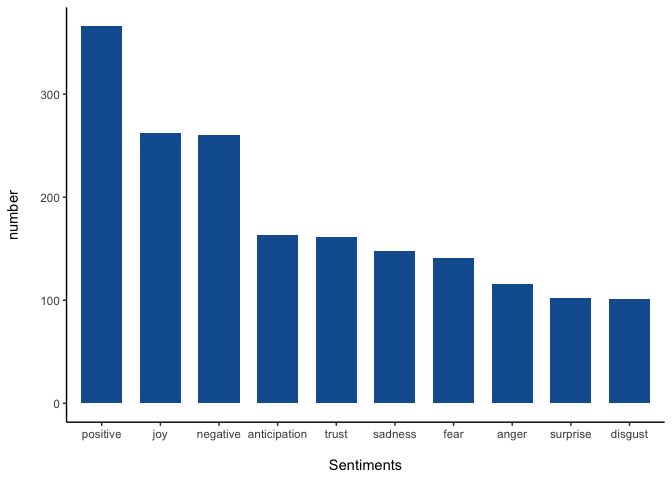
Sentiment analysis of titles
In order to analyze the sentiment of the words in the titles, I got the
stop words(meaningless words) dictionary and sentiment dictionary from
the tidytext library.
sentiments <- get_sentiments("nrc")

df_sentiments <- title_words %>%
  filter(word != "") %>%
  anti_join(stop_words,by = "word") %>%
  left_join(sentiments)
df_sentiments_filtered <- df_sentiments %>%
  filter(!is.na(sentiment)) %>%
  group_by(sentiment) %>%
  summarize(n = n()) %>%
  arrange(desc(n))
After removed the stop word, I counted the number of each word in the titles.
df_sentiments_filtered %>%
  ggplot(aes(x = reorder(sentiment, n, function(n) -n), y = n)) +
  geom_bar(stat = "identity",fill="#125FA0", width = 0.7) +
  theme_classic() +
  labs(x = "\nSentiments", y="number\n")
And we can also count what is the percentage of positive words in the words that have sentiments.
words_positive <- df_sentiments %>%
  filter(sentiment == "positive") %>%
  group_by(word) %>%
  summarise(n=n())

words_all_sentiment <- df_sentiments %>%
  filter(!is.na(sentiment)) %>%
  group_by(word) %>%
  summarize(n = n()) %>%
  arrange(desc(n))

nrow(words_positive)/nrow(words_all_sentiment)
## [1] 0.4294671
Who spent the most weeks at #1 for the decade 2000-2009?
df %>%
  group_by(artist) %>%
  summarise(top1_time_sum = sum(weeks_at_number_1)) %>%
  arrange(desc(top1_time_sum)) %>%
  head(1)
## # A tibble: 1 x 2
##   artist         top1_time_sum
##   <chr>                  <int>
## 1 JACKSON, JANET            39
And there are the songs belong to this artist.
df %>%
  filter(artist == "JACKSON, JANET",
         weeks_at_number_1 != 0) %>%
  arrange(desc(weeks_at_number_1)) %>%
  select(song_title, artist, year, weeks_at_number_1)
## # A tibble: 6 x 4
##   song_title                            artist       year  weeks_at_number…
##   <chr>                                 <chr>        <fct>            <int>
## 1 SOMEONE TO CALL MY LOVER              JACKSON, JA… 2001                10
## 2 ALL FOR YOU                           JACKSON, JA… 2001                10
## 3 "DOESN'T REALLY MATTER (from \"NUTTY… JACKSON, JA… 2000                 8
## 4 FEEDBACK                              JACKSON, JA… 2008                 6
## 5 SPECIAL                               JACKSON, JA… 2000                 3
## 6 LUV                                   JACKSON, JA… 2008                 2
What song spent the most weeks at #1 for the decade 2000-2009?
df %>%
  arrange(desc(weeks_at_number_1)) %>%
  select(song_title, artist, year, weeks_at_number_1) %>%
  head(1)
## # A tibble: 1 x 4
##   song_title    artist      year  weeks_at_number_1
##   <chr>         <chr>       <fct>             <int>
## 1 NO SUCH THING MAYER, JOHN 2002                 13
What song peaked at #1 the quickest in the decade 2000-2009?
df %>%
  filter(weeks_at_number_1 != 0) %>%
  arrange(weeks_to_reach_peak) %>%
  select(song_title, artist, year, weeks_at_number_1, weeks_to_reach_peak, debut_date, peak_date) %>%
  head(1)
## # A tibble: 1 x 7
##   song_title artist year  weeks_at_number… weeks_to_reach_… debut_date
##   <chr>      <chr>  <fct>            <int>            <int> <date>
## 1 SOMEONE T… JACKS… 2001                10                2 2001-07-22
## # … with 1 more variable: peak_date <date>
What song took the longest to reach #1 in the decade 2000-2009?
df %>%
  filter(weeks_at_number_1 != 0) %>%
  arrange(desc(weeks_to_reach_peak)) %>%
  select(song_title, artist, year, weeks_at_number_1, weeks_to_reach_peak, debut_date, peak_date) %>%
  head(1)
## # A tibble: 1 x 7
##   song_title artist year  weeks_at_number… weeks_to_reach_… debut_date
##   <chr>      <chr>  <fct>            <int>            <int> <date>
## 1 BEFORE HE… UNDER… 2007                 3               31 2006-11-05
## # … with 1 more variable: peak_date <date>
Solo men, solo women, groups for the decade 2000-2009 - design a graphic that shows the distribution of songs hitting #1
The solo artists have their full name in the data by the format as “LastName, FirstName”, as a result, we can tell whether the data is a single person name by the presence of a comma.
df %>%
  mutate(solo_group = case_when(str_detect(string = artist, pattern = ",") ~ "solo",
                                TRUE ~ "group")) %>%
  mutate(solo_group = as.factor(solo_group)) %>%
  filter(weeks_at_number_1 != 0) %>%
  group_by(solo_group) %>%
  summarise(number = n())
## # A tibble: 2 x 2
##   solo_group number
##   <fct>       <int>
## 1 group          92
## 2 solo           84
Actually, there is no built-in pie chart function in ggplot2. But we
can use bar chart function then twisting the y-axis to the polar
coordinate system to create a pie chart.
df %>%
  mutate(solo_group = case_when(str_detect(string = artist, pattern = ",") ~ "solo",
                                TRUE ~ "group")) %>%
  mutate(solo_group = as.factor(solo_group)) %>%
  filter(weeks_at_number_1 != 0) %>%
  ggplot()+
  geom_bar(aes(x=1, fill = solo_group))+
  coord_polar(theta = "y")+
  theme(axis.text = element_blank(),
        axis.title = element_blank(),
        axis.ticks = element_blank(),
        axis.line = element_blank(),
        legend.title = element_blank(),
        panel.background = element_blank()
        )+
  scale_fill_brewer(palette = "Paired")

Solo men, solo women, groups for the decade 2000-2009 - design a graphic that shows the distribution of songs hitting the Top 10
df %>%
  mutate(solo_group = case_when(str_detect(string = artist, pattern = ",") ~ "solo",
                                TRUE ~ "group")) %>%
  mutate(solo_group = as.factor(solo_group)) %>%
  filter(weeks_top_10 != 0) %>%
  group_by(solo_group) %>%
  summarise(number = n())
## # A tibble: 2 x 2
##   solo_group number
##   <fct>       <int>
## 1 group         318
## 2 solo          255
df %>%
  mutate(solo_group = case_when(str_detect(string = artist, pattern = ",") ~ "solo",
                                TRUE ~ "group")) %>%
  mutate(solo_group = as.factor(solo_group)) %>%
  filter(weeks_top_10 != 0) %>%
  ggplot()+
  geom_bar(aes(x=1, fill = solo_group))+
  coord_polar(theta = "y")+
  theme(axis.text = element_blank(),
        axis.title = element_blank(),
        axis.ticks = element_blank(),
        axis.line = element_blank(),
        legend.title = element_blank(),
        panel.background = element_blank()
        )+
  scale_fill_brewer(palette = "Paired")

What song spent the most time on the charts in the decade 2000-2009)
df %>%
  arrange(desc(weeks_top_50)) %>%
  select(song_title, artist, year, weeks_top_50) %>%
  head(3)
## # A tibble: 3 x 4
##   song_title                      artist                 year  weeks_top_50
##   <chr>                           <chr>                  <fct>        <int>
## 1 TIME OF YOUR LIFE (GOOD RIDDAN… GREEN DAY              2006            65
## 2 BEFORE HE CHEATS                UNDERWOOD, CARRIE      2007            57
## 3 GLAMOROUS                       FERGIE featuring LUDA… 2007            50
Actually, TIME OF YOUR LIFE (GOOD RIDDANCE) never be the top 1. A sad story.
Is there a correlation between weeks spent on the chart and weeks at #1?
cor(x = df[["weeks_at_number_1"]],
    y = df[["weeks_top_50"]])
## [1] 0.471703
df %>%
  ggplot(aes(x=weeks_at_number_1, y=weeks_top_50))+
  geom_jitter(alpha = 0.3, color = "dodgerblue4")+
  geom_smooth(color = "dodgerblue4", se = FALSE)+
  theme_classic()+
  labs(x="\nWeeks at Top 1", y="Weeks at Top 50\n")

Hint: Project GitHub page: Cashbox-Magazine-song-records-Analysis