Absolute error and relative error have a little bit different on calculation but the difference really makes an essential change. The absolute error will be influenced by the sample size but relative error can show the real error without huge bias.
when used as a measure of precision—is the ratio of the absolute error of a measurement to the measurement being taken. In other words, this type of error is relative to the size of the item being measured. RE is expressed as a percentage and has no units.
From Statistics How To
Absolute Error
absolute error = |p̂−p|
The difference between the measured or inferred value of a quantity x_0 and its actual value x.
Let’s create a table to save 14*5 results of our simulation first.
n <- rep(NA, 14)
for(i in 1:14){n[i] <- 2^(i+1)}
T <- matrix(NA,14,5)
p <- c(0.01,0.05,0.10,0.25,0.5)
Then generate 1 or 0 randomly for 1000 times for each situation and calculate the absolute error.
for(x in 1:length(p)){
  for(y in 1:length(n)){
    TS <- rep(NA,10000)
    for(m in 1:10000){
      TS[m] <- abs(rbinom(1,n[y],p[x])/n[y]-p[x])
    }
    T[y,x] <- mean(TS)
  }
}
Change the y-scale to log_10.
T <- log10(T)
In the end, plot the graph to show the relationship between p and absolute error.
plot(T[,5],xlim=c(0,14),ylim=range(T),col="red",type="b",xaxt="n",xlab="N(log_2 scale)",ylab="Absolute Error",pch=16, lwd=3)
lines(T[,2],col="purple",type="b",pch=16, lwd=3)
lines(T[,3],col="blue",type="b",pch=16, lwd=3)
lines(T[,4],col="green",type="b",pch=16, lwd=3)
lines(T[,1],col="gray",type="b",pch=16, lwd=3)

lname <- c("0.01","0.05","0.10","0.25","0.50")
lname_p <- paste0("p = ",lname)
xname <- c("4","8","16","32","64","128","256","512","1024","2048","4096","8192","16384","32768")

axis(1, at=1:14,las=2, lab=xname)
text(1,T[1,],lname_p,pos=2,cex=0.6)
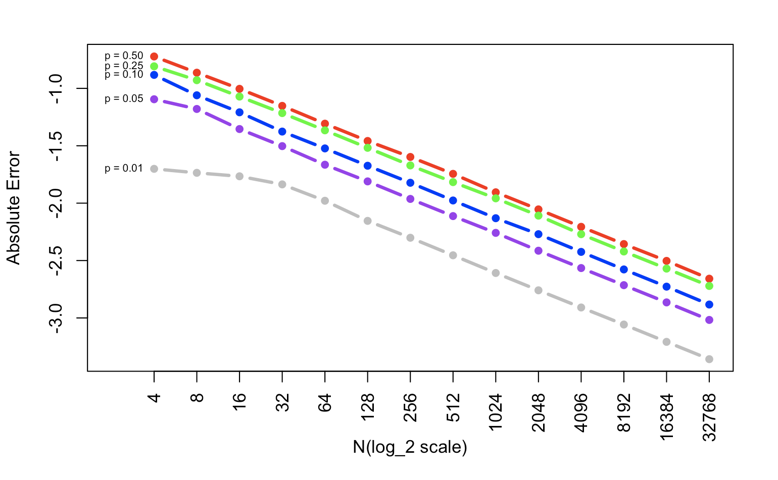
Absolute error is just the absolute value of the value you have the minus expected value. In this simulation, you calculated the absolute error 10000 times and get the mean value of them in every situation. When we transfer the y scale to log_10, it is obvious that the x & y have a linear connection. The p is higher, the absolute error is bigger.
Relative Error
Relative error = |p̂−p|/p.
Then do the same thing as before but when we calculate the error, use absolute error divide by p-value. Plot the graph too.
n <- rep(NA, 14)
for(i in 1:14){n[i] <- 2^(i+1)}

T2 <- matrix(NA,14,5)
p <- c(0.01,0.05,0.10,0.25,0.5)

for(x in 1:length(p)){
  for(y in 1:length(n)){
    T2S <- rep(NA,10000)
    for(m in 1:10000){
      T2S[m] <- abs(rbinom(1,n[y],p[x])/n[y]-p[x])/p[x]
    }
    # T2[y,x] <- abs(rbinom(1,n[y],p[x])/n[y]-p[x])/p[x]
    T2[y,x] <- mean(T2S)
  }
}

T2 <- log10(T2)

xname <- c("4","8","16","32","64","128","256","512","1024","2048","4096","8192","16384","32768")
lname <- c("0.01","0.05","0.10","0.25","0.50")
lname_p <- paste0("p = ",lname)

plot(T2[,1],xlim=c(0,14),ylim=range(T2),col="red",type="b",pch=16,xaxt="n",xlab="N(log_2 scale)",ylab="Relative Error", lwd=3)
lines(T2[,2],col="purple",type="b",pch=16, lwd=3)
lines(T2[,3],col="blue",type="b",pch=16, lwd=3)
lines(T2[,4],col="green",type="b",pch=16, lwd=3)
lines(T2[,5],col="gray",type="b",pch=16, lwd=3)
axis(1, at=1:14,las=2, lab=xname)
text(1,T2[1,],lname_p,pos=2,cex=0.6)
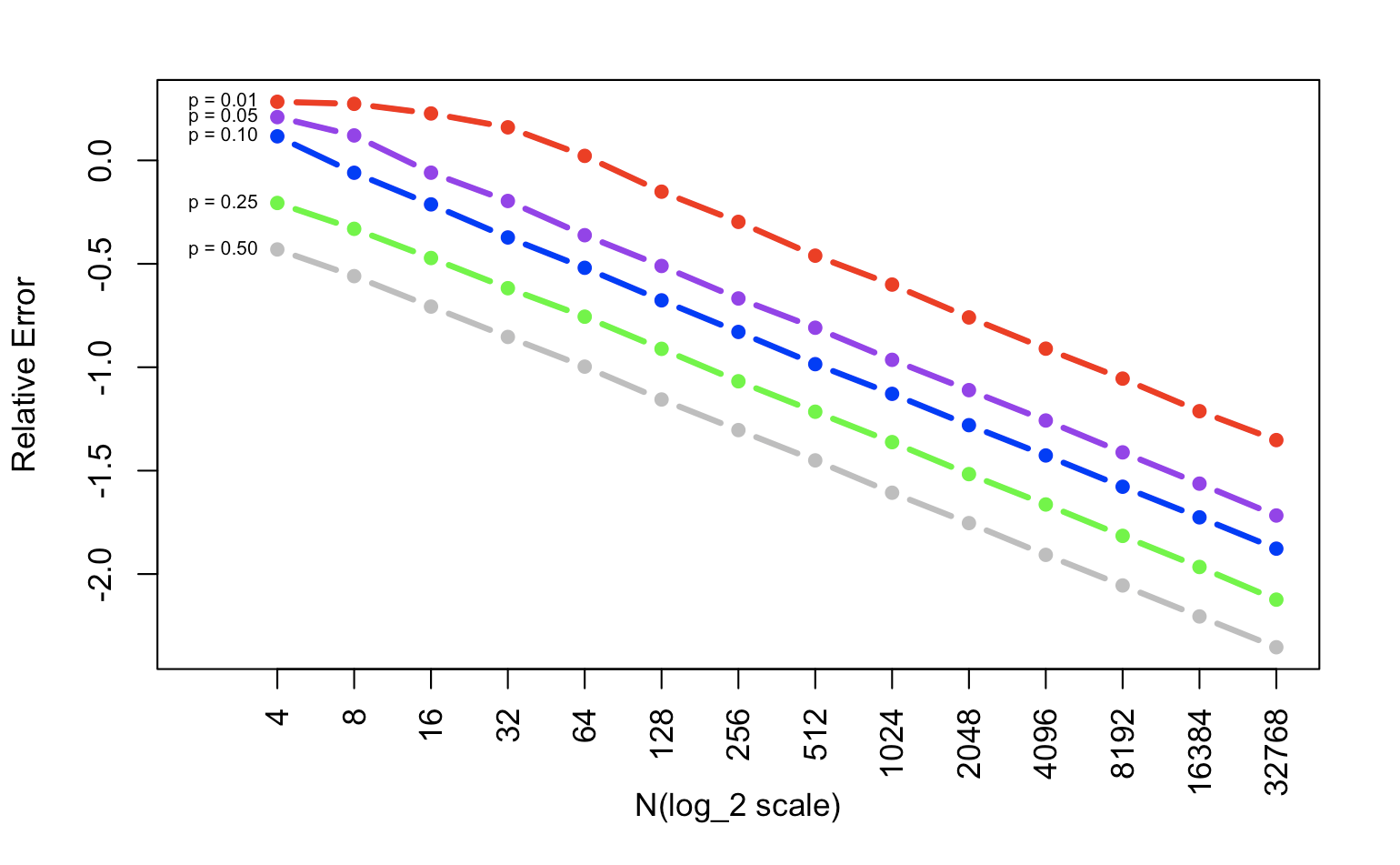
Again, compare with absolute error, if you want to calculate relative error, the only thing you need to do is use the absolute error divided by p, the value you have. This process keeps the influence of the value size and focuses on the error itself. When we change the y scale into log_10, the xy relationship is also linear. But the bigger p we have, the smaller relative error we get.